 Credit: Dreamstime
While machine learning and deep learning models often produce good classifications and predictions, they are almost never perfect. Models almost always have some percentage of false positive and false negative predictions. That’s sometimes acceptable, but matters a lot when the stakes are high. For example, a drone weapons system that falsely identifies a school as a terrorist base could inadvertently kill innocent children and teachers unless a human operator overrides the decision to attack.
The operator needs to know why the AI classified the school as a target and the uncertainties of the decision before allowing or overriding the attack. There have certainly been cases where terrorists used schools, hospitals, and religious centers as bases for missile attacks. Was this school one of those? Is there intelligence or a recent observation that identifies the school as currently occupied by such terrorists? Are there reports or observations that establish that no students or teachers are present in the school?
If there are no such explanations, the model is essentially a black box, and that’s a huge problem. For any AI decision that has an impact — not only a life and death impact, but also a financial impact or a regulatory impact — it is important to be able to clarify what factors went into the model’s decision.
What is explainable AI?
Explainable AI (XAI), also called interpretable AI, refers to machine learning and deep learning methods that can explain their decisions in a way that humans can understand. The hope is that XAI will eventually become just as accurate as black-box models.
Explainability can be ante-hoc (directly interpretable white-box models) or post-hoc (techniques to explain a previously trained model or its prediction). Ante-hoc models include explainable neural networks (xNNs), explainable boosting machines (EBMs), supersparse linear integer models (SLIMs), reversed time attention model (RETAIN), and Bayesian deep learning (BDL).
Post-hoc explainability methods include local interpretable model-agnostic explanations (LIME) as well as local and global visualisations of model predictions such as accumulated local effect (ALE) plots, one-dimensional and two-dimensional partial dependence plots (PDPs), individual conditional expectation (ICE) plots, and decision tree surrogate models.
How XAI algorithms work
If you followed all the links above and read the papers, more power to you – and feel free to skip this section. The write-ups below are short summaries. The first five are ante-hoc models, and the rest are post-hoc methods.
Explainable neural networks
Explainable neural networks (xNNs) are based on additive index models, which can approximate complex functions. The elements of these models are called projection indexes and ridge functions. The xNNs are neural networks designed to learn additive index models, with subnetworks that learn the ridge functions. The first hidden layer uses linear activation functions, while the subnetworks typically consist of multiple fully-connected layers and use nonlinear activation functions.
xNNs can be used by themselves as explainable predictive models built directly from data. They can also be used as surrogate models to explain other nonparametric models, such as tree-based methods and feedforward neural networks. The 2018 paper on xNNs comes from Wells Fargo.
Explainable boosting machine
As I mentioned when I reviewed Azure AI and Machine Learning, Microsoft has released the InterpretML package as open source and has incorporated it into an Explanation dashboard in Azure Machine Learning. Among its many features, InterpretML has a “glassbox” model from Microsoft Research called the explainable boosting machine (EBM).
EBM was designed to be as accurate as random forest and boosted trees while also being easy to interpret. It’s a generalised additive model, with some refinements. EBM learns each feature function using modern machine learning techniques such as bagging and gradient boosting. The boosting procedure is restricted to train on one feature at a time in round-robin fashion using a very low learning rate so that feature order does not matter. It can also detect and include pairwise interaction terms. The implementation, in C++ and Python, is parallelisable.
Supersparse linear integer model
Supersparse linear integer model (SLIM) is an integer programming problem that optimises direct measures of accuracy (the 0-1 loss) and sparsity (the l0-seminorm) while restricting coefficients to a small set of coprime integers. SLIM can create data-driven scoring systems, which are useful in medical screening.
Reverse time attention model
The reverse time attention (RETAIN) model is an interpretable predictive model for electronic health records (EHR) data. RETAIN achieves high accuracy while remaining clinically interpretable. It’s based on a two-level neural attention model that detects influential past visits and significant clinical variables within those visits (e.g. key diagnoses). RETAIN mimics physician practice by attending the EHR data in a reverse time order so that recent clinical visits are likely to receive higher attention. The test data discussed in the RETAIN paper predicted heart failure based on diagnoses and medications over time.
Bayesian deep learning
Bayesian deep learning (BDL) offers principled uncertainty estimates from deep learning architectures. Basically, BDL helps to remedy the issue that most deep learning models can’t model their uncertainty by modeling an ensemble of networks with weights drawn from a learned probability distribution. BDL typically only doubles the number of parameters.
Local interpretable model-agnostic explanations
Local interpretable model-agnostic explanations (LIME) is a post-hoc technique to explain the predictions of any machine learning classifier by perturbing the features of an input and examining the predictions. The key intuition behind LIME is that it is much easier to approximate a black-box model by a simple model locally (in the neighborhood of the prediction we want to explain), as opposed to trying to approximate a model globally. It applies both to the text and image domains. The LIME Python package is on PyPI with source on GitHub. It’s also included in InterpretML.
 Christoph Molnar
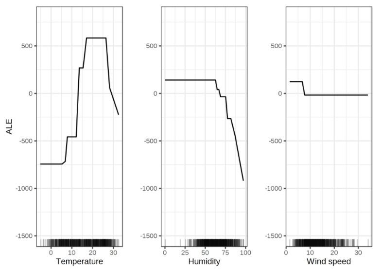
ALE plots for bicycle rentals. From Interpretable Machine Learning by Christoph Molnar.
Accumulated local effects
Accumulated local effects (ALE) describe how features influence the prediction of a machine learning model on average, using the differences caused by local perturbations within intervals. ALE plots are a faster and unbiased alternative to partial dependence plots (PDPs). PDPs have a serious problem when the features are correlated. ALE plots are available in R and in Python.
 Christoph Molnar
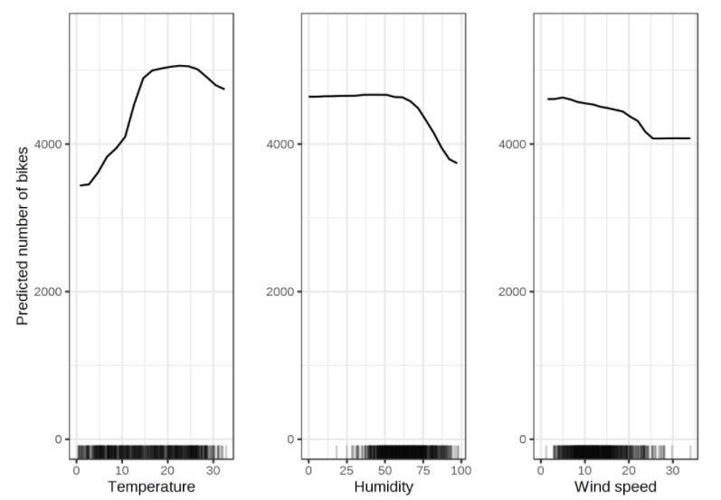
PDP plots for bicycle rentals. From Interpretable Machine Learning by Christoph Molnar.
Partial dependence plots
A partial dependence plot (PDP or PD plot) shows the marginal effect one or two features have on the predicted outcome of a machine learning model, using an average over the dataset. It’s easier to understand PDPs than ALEs, although ALEs are often preferable in practice. The PDP and ALE for a given feature often look similar. PDP plots in R are available in the iml, pdp, and DALEX packages; in Python, they are included in Scikit-learn and PDPbox.
 Christoph Molnar
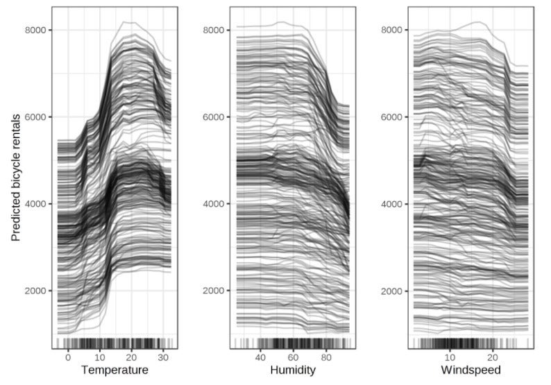
ICE plots for bicycle rentals. From Interpretable Machine Learning by Christoph Molnar. CC
Individual conditional expectation plots
Individual conditional expectation (ICE) plots display one line per instance that shows how the instance’s prediction changes when a feature changes. Essentially, a PDP is the average of the lines of an ICE plot. Individual conditional expectation curves are even more intuitive to understand than partial dependence plots. ICE plots in R are available in the iml, ICEbox, and pdp packages; in Python, they are available in Scikit-learn.
Surrogate models
A global surrogate model is an interpretable model that is trained to approximate the predictions of a black box model. Linear models and decision tree models are common choices for global surrogates.
To create a surrogate model, you basically train it against dataset features and the black box model predictions. You can evaluate the surrogate against the black box model by looking at the R-squared between them. If the surrogate is acceptable, then you can use it for interpretation.
Read more on the next page...


